Week 4
Causality
Soci—316
Qualtrics Survey Assessment Deadline
Your Qualtrics survey assignment is now due by 8:00 PM on Monday, March 2nd.
Social scientists are often interested in drawing causal inferences.
X \to Y
About what, exactly? There are a dizzying array of examples.
Here are three questions that invite causal claims:
Do smaller class sizes improve pedagogical outcomes?
Will investments in family planning programs improve economic and health outcomes for women in low-income settings?
Did the cultural grievances of the “middle class” trigger the rise of fascist politics in interwar Europe?
Let’s pause for a second.
Try to frame your research question in causal terms.
Rearrange the text in the box below to arrive at your question.
We can, of course, deploy quantitative tools (e.g., estimators, weighting, causal diagrams, experiments) to “resolve” causal questions—or at least adduce evidence grounded in statistical reasoning.
For an overview of how causality “works” in ethnographic research, see Small (2013).
Let’s assume that our outcomes of substantive interest are approximately linear. Can we estimate linear regression models to “resolve”
our causal questions?
y = \beta_0 + \beta_1 x + \epsilon
Click to Expand Image & Launch Two-DAG Gallery
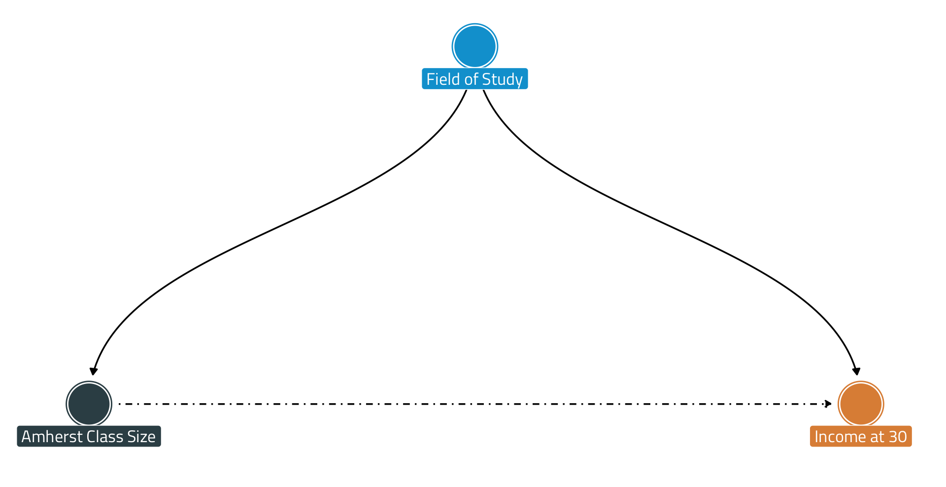
How can we deal with confounding—i.e., to estimate the causal effect of class size at Amherst on post-graduate outcomes?
Randomization is the gold standard.
We will return to this point in a second.
Causal relationships refer to the cause-and-effect connection between two variables … We refer to the variable where the change originates as the treatment variable. We refer to the variable that may change in response to the change in the treatment variable as the outcome variable.
(Llaudet and Imai 2023:28, EMPHASIS ADDED)
small_i= \begin{cases} 1 & \text{if individual } i \text{ assigned to small classes at Amherst}\\ 0 & \text{if individual } i \text{ was not assigned to small classes at Amherst} \end{cases}
When estimating the causal effect of X on Y, we attempt to quantify the change in the outcome variable Y that is caused by a change in the treatment variable X … In mathematical notation, we represent change with \Delta (the Greek letter Delta), and thus, we represent a change in the outcome as \Delta Y. To measure this change in the outcome Y, ideally we would compare two potential outcomes: the outcome when the treatment is present and the outcome when the treatment is absent.
(Llaudet and Imai 2023:29–30, EMPHASIS ADDED)
Y_{i}(X_{i}=1) is the potential outcome under the treatment condition for individual i (the value of Y_{i} if X_{i}=1).
Y_{i}(X_{i}=0) is the potential outcome under the control condition for individual i (the value of Y_{i} if X_{i}=0).
(Llaudet and Imai 2023:30, EMPHASIS ADDED)
\Delta income_{i} = \underbrace{income_{i}\!\left(small_{i}=1\right)}_{\text{Treatment}} - \underbrace{income_{i}\!\left(small_{i}=0\right)}_{\text{Control}}
\textit{Individual Effect}_i \;=\; \Delta Y_i \;=\; Y_i(X_i=1) \;-\; Y_i(X_i=0)
Adaptation of summary box in Llaudet and Imai (2023:30).
Unfortunately, this kind of analysis is not possible. In the real world, we never observe both potential outcomes for the same individual. Instead, we observe only the factual outcome, which is the potential outcome under whichever condition (treatment or control) was received in reality. We can never observe the counterfactual outcome, which is the potential outcome that would have occurred under whichever condition (treatment or control) was not received in reality. As a result, we cannot compute causal effects at the individual level.
(Llaudet and Imai 2023:32, EMPHASIS ADDED)
Adaptation of summary box in Llaudet and Imai (2023:33).
Alas, this can’t happen in real life for person i

Image can be retrieved here.
To get around the fundamental problem of causal inference, we must find good approximations for the counterfactual outcomes. To accomplish this, we move away from individual-level effects and focus on the average causal effect across a group of individuals.
The average causal effect of the treatment X on the outcome Y, also known as the average treatment effect, is the average of all the individual causal effects of X on Y within a group. Since each individual causal effect is the change in Y caused by a change in X for a particular individual, the average causal effect of X on Y is the average change in Y caused by a change in X for a group of individuals.
(Llaudet and Imai 2023:33, EMPHASIS ADDED)
Adaptation of summary box in Llaudet and Imai (2023:34).
How can we obtain good approximations for the counterfactual outcomes, which by definition cannot be observed? As we will see in detail soon, we must find or create a situation in which the treated observations and the untreated observations are similar with respect to all the variables that might affect the outcome other than the treatment variable itself. The best way to accomplish this is by conducting a randomized experiment.
(Llaudet and Imai 2023:34, EMPHASIS ADDED)
In a randomized experiment, also known as a randomized controlled trial (RCT), researchers decide who receives the treatment based on a random process …
(Llaudet and Imai 2023:34, EMPHASIS ADDED)
| Group | Treatment | Control | Δ |
|---|
When treatment assignment is randomized, the only thing that distinguishes the treatment group from the control group, besides the reception of the treatment, is chance. This means that although the treatment and control groups consist of different individuals, the two groups are comparable to each other, on average, in all respects other than whether or not they received the treatment.
Random treatment assignment makes the treatment and control groups on average identical to each other in all observed and unobserved pre-treatment characteristics. Pre-treatment characteristics are the characteristics of the individuals in a study before the treatment is administered.
(Llaudet and Imai 2023:36, EMPHASIS ADDED)
Adaptation of summary box in Llaudet and Imai (2023:36).
With randomization, this holds for two populations, C (X_{i}=0) and T (X_{i}=1)
Image can be retrieved here.
If the treatment and control groups were comparable before the treatment was administered … we can use the factual outcome of one group as an approximation for the counterfactual outcome of the other. In other words, we can assume that the average outcome of the treatment group is a good estimate of the average outcome of the control group, had the control group received the treatment. Similarly, we can assume that the average outcome of the control group is a good estimate of the average outcome of the treatment group, had the treatment group not received the treatment. As a result, we can approximate the average treatment effect by computing the difference in the average outcomes between the treatment and control groups. Since both of these average outcomes are observed, this is an analysis we are able to perform.
(Llaudet and Imai 2023:37, EMPHASIS ADDED)
Adaptation of summary box in Llaudet and Imai (2023:37).
Adaptation of summary box in Llaudet and Imai (2023:38).
As Llaudet and Imai (2023:38) note, social scientists often run into ethical, logistical, and financial obstacles that ensure that fielding a randomized experiment is challenging—if not impossible.
With this in mind, think about—and refine—your own causal question once again. Can you randomly sort respondents into C (X_{i}=0) and T (X_{i}=1)? How might you go about doing so? What are some challenges you may run into?
Why might class size at Amherst College be correlated with an alum’s income at age 30?
Field of Study is a confounder in this instance.